1) Source Representations. The Khamisiyah dispersion calculations required characterizing the source term, including the emission’s location, time, strength, and duration. As described earlier, the initial release took place at 30� 44’32"N, 46� 25’52"E at 1315 UTC on March 10, 1991. The tests conducted at Dugway and subsequent analysis predicted that the detonation released 32% of the available chemical warfare agent, most of it leaking into the soil and wood. Out of this 32%, 18% entered the atmosphere-2% through immediate aerosolization and 16% through evaporation (5.75% from soil and 10.4% from wood). Moreover, as Figure A-23 showed, most of the chemical warfare agent evaporated during the first ten hours.

To characterize the source term, the CIA made these assumptions:

• The initial distribution of the agent mass was according to the description in IV.B.1.d and shown in Figure A-22;
• The total agent evaporation rate was produced by combining the Dugway-generated rates for specific agent environments (e.g., GB evaporation from soil, GF evaporation from wood, etc.). When combined, these data provide the total agent mass flux shown in Figure A-23;
• Since the Dugway field test results and subsequent analysis estimated the mass released as a function of time, the models’ internal surface evaporation algorithms were not used, except for the July 1997 VLSTRACK run. That model run was completed before NSWC received the Dugway source data. Consequently, NSWC used internal VLSTRACK evaporation algorithms to estimate the source term. All subsequent VLSTRACK calculations used the Dugway source data.
• In 1997, the GB/GF mixture was treated as a single agent, since GB and GF’s toxicity values were assumed equal; and
• Table A-11 below describes the initial configuration of the agent cloud assumed for VLSTRACK and HPAC/SCIPUFF.

	Release Location	Release Frequency	Initial Cloud Sigmas	Vertical Centroid of Initial Cloud
VLSTRACK	Thirteen individual puffs released as volume sources at the stack locations shown in Figure A-3. The mass distribution as determined by the methods described above is scaled for each stack size.	15 min	x = 6m y = 6m z = 6m	1m
HPAC/ SCIPUFF	Ten volume sources were used to represent the contributions of all 13 stacks released at the nominal location:	15 min	x = 30m y = 30m z = 10m	1m

2) Model parameterizations. Certain atmospheric conditions (photolysis, hydrolysis, gas-phase reactions, and thermal decomposition) degrade GB and GF, but these effects were not specifically included in the modeling, a decision the IDA panel endorsed because of the lack of well-established empirical data on which to base such parameterizations. For the July 1997 Khamisiyah analysis, DoD’s two dispersion models, VLSTRACK and HPAC/SCIPUFF, treated dry deposition of GB and GF vapor in a default manner. VLSTRACK neglected dry deposition altogether. HPAC/SCIPUFF represented dry deposition with the deposition velocity V_d. The default value of 0.3 cm/s for GB in the HPAC/SCIPUFF material database was used. Including degradation effects would decrease the amount of chemical agent in the atmosphere. Not incorporating these degradation effects kept the simulated agent levels at full potency and produced a higher predicted concentration.

3) Dosages, Concentrations, and Limits. In 1997, the possible exposures from the dispersion of the GB-GF mixture were estimated with the toxicity properties of GB only. To satisfy the PAC’s requests, two levels of possible exposure were considered. Both exposure levels are represented in terms of dosage (the concentration of agent to which a person is exposed over a specific period of time).

• First noticeable effects or FNE (1 mg-min/m³). This dosage likely would cause watery eyes, runny nose, chest tightness, muscle twitching, sweating, and headache. Increasingly higher dosages would impair vision, incapacitate, and possibly kill.
  
  
• General population limit or GPL (0.01296 mg-min/m³). This dosage indicates the limit below which the general population, including children and older people, could remain exposed for 72 hours without any adverse effects. This amount is derived from a maximum averaged air concentration of 0.000003 mg/m³ allowable for the general population over 72 hours.

To appreciate the magnitude of difference between the levels, note the general population limit dosage (0.01296 mg-min/m³) is 1/80 the dosage expected to produce noticeable effects (1 mg-min/m³). The area between these levels, which the 1997 modeling called the area of low-level exposure, is the one that requires more medical research. The exposure time at Khamisiyah was relatively brief, measured in hours, not weeks as would be the case with low-level occupational exposures.

4) Reconstructing the Vapor Cloud Using Several Model Results. To address concerns about model uncertainty, the DoD/CIA modeling team adopted a methodology combining the results of four different meteorological and dispersion simulations. That is, to define the extent of the hazard area, the union of the contour areas predicted by all simulations is considered. These four simulations include:

• COAMPS Experiment 4 (based on NOGAPS), coupled with HPAC/SCIPUFF;
• OMEGA (based on GDAS), coupled with HPAC/SCIPUFF;
• MM5 (based on ECMWF), coupled with HPAC/SCIPUFF; and
• COAMPS Experiment 4 (based on NOGAPS), coupled with VLSTRACK.

The results from an OMEGA/NUSSE4 simulation were also incorporated for confirmatory purposes only.

HPAC/SCIPUFF predicts concentration means as well as variances. With an assumed clipped-normal probability distribution function (Lewellen and Sykes, 1986), the means and variances were used to probabilistically estimate concentrations and dosages. The clipped normal distribution was obtained by replacing all negative values in a general Gaussian distribution with zeros. The HPAC/SCIPUFF results were based on the 1% probability contours, i.e., at any point along the contour of value A, the probability that the dosage there is higher than A is 1%. The 1% probability contours always cover a larger area than do median (50%) probability contours. Traditional dispersion models, such as VLSTRACK, predict only median concentrations and dosages.

DoD used several databases in conjunction with dispersion model results to determine unit locations and their possible exposure from the Khamisiyah Pit demolitions.

1) US Armed Services Center for Unit Records Research. In 1993, DoD tasked the US Armed Services Center for Unit Records Research (USASCURR), formerly the US Armed Services Center for Research of Unit Records, located at the Fort Belvoir Engineer Proving Ground, VA, to develop the DoD Persian Gulf Unit Movement Database to capture geographic locations for Army, Navy, Marine Corps, Air Force, and Coast Guard units throughout the Operation Desert Storm theater of operations. USASCURR gathered unit location information from a wide range of sources, including unit history data archives, operational logs and situation reports, after-action reports, and other historical files. These sources amounted to more than 5 million pieces of paper from which USASCURR created over 600,000 unit grid coordinates. USASCURR established and followed a rigorous quality assurance program to ensure data were correctly entered according to the source document. From April to June 1997, Army brigade and division operations officers from XVIII Airborne Corps, the major subordinate command near Khamisiyah during March 1991, came to USASCURR to review, refine, and enhance the resolution and accuracy of the unit location information in the database. The availability of the unit location data was a fundamental step that enabled the US Army Center for Health Promotion and Preventive Medicine (USACHPPM) to determine the units within the possible hazard areas.

2) Defense Manpower Data Center. The Defense Manpower Data Center (DMDC) database contains roughly 700,000 records of in-theater personnel, containing not only a servicemember’s last assigned Unit Identification Code (UIC), but also lists of UICs for six distinct time frames for active duty personnel and two additional time frames for reserve units. The DMDC database identifies by social security number specific personnel assigned to the units in the USASCURR database.

3) Vapor Cloud Outputs. USACHPPM received HPAC/SCIPUFF and VLSTRACK dispersion model summary results for March 10-13, 1991. The model summary results included daily text files that show the longitudinal and latitudinal coordinates outlining the applicable agent-dosage contours (Table A-12.) In addition to the FNE and GPL thresholds previously defined, USACHPPM also included the threshold for the M8A1 chemical warfare agent detector alarm to sound. The outlines of these hazard contours together with the USASCURR database determine which troop units were in the hazard areas.

4) Identifying Individual Servicemembers Possibly Exposed to Nerve Agent. USACHPPM prepared a base map for the Desert Storm theater of operations on which it overlaid the troop units’ daily locations (by UIC) provided by USASCURR and the HPAC/SCIPUFF and VLSTRACK dispersion model results for March 10 through 13, 1991. Based upon the overlay of the threshold contours’ boundaries with daily unit locations and the assumption that the servicemembers were with their assigned units on that day and at that location, USACHPPM identified the units by UIC, which the Office of the Special Assistant then used the DMDC database to identify individual servicemembers possibly exposed.

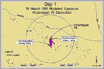
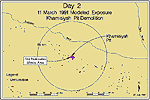
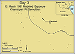
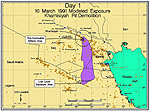
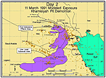
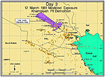
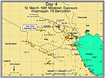
5) Results. Figures A-51 through A-57 show the union dosage contours from all four simulations for each day from March 10 to 13, 1991, overlaid with unit locations (shown as brown dots) for that day. This methodology identifies any unit included in contours produced by at least one of the four simulations as possibly having been exposed. For each daily plot, dosages had been accumulated daily (24 hours) except for first and last days.

Figures A-51 through A-53 show dosage contours representing acute (first noticeable effects) levels from the early stages of evaporation from the wood and soil, characterized by relatively high mass flux. Northerly winds prevailed during the first day and hence downwind dispersion extended acute levels approximately 20 km to the south (Figure A-51). According to the USACHPPM overlays, no troops were located in these areas south of Khamisiyah on March 10, 1991; hence, no acute exposures occurred. The winds diminished on the second day. Figure A-52 shows that the acute dosage contour for the second day lies essentially within that of the first day. Evaporation rates diminish rapidly over the last two days (March 12-13, 1991), reflected in Figure A-53, which shows dosage levels falling below the acute level on the third day. Consequently, the modeling results predicted no exposure to acute levels for any units due to the release of chemical warfare agent at Khamisiyah.

Figure A-51. 1997 FNE hazard assessent for March 10, 1991

Figure A-52. 1997 FNE hazard assessment for March 11, 1991

FigureA-53. 1997 FNE hazard assessment for March 12, 1991

Figures A-54 through A-57 show the daily general population limit dosage contours. Northerly winds on March 10, 1991, produced a vapor cloud extending through western Kuwait and across the Saudi Arabian border. During the second day, although winds generally were calm near Khamisiyah, easterly winds carried the vapor cloud to the west-southwest. On the third day, winds dispersed the evaporating chemical warfare agent to the west-northwest near the Pit. Decaying soil and wood evaporation rates and calm winds limited dispersion on the fourth day.

Figure A-54. 1997 GPL hazard (low-level exposure) assessment for March 10, 1991

Figure A-55. 1997 GPL hazard (low-level exposure) assessment for March 11, 1991

Figure A-56. 1997 GPL hazard (low-level exposure) assessment for March 12, 1991

Figure A-57. 1997 GPL hazard (low-level exposure) assessment for March 13, 1991